nn_tuning
Analyse neural networks for feature tuning.
Installing and configuring nn_tuning
Install nn_analysis using the following pip command. This requires python > 3.6.
$ pip install nn_tuning
If you wish to use the plotting functions in any of the classes, you need to install Matplotlib. To do so you can use the following command:
$ pip install matplotlib
Depending on the type of neural network you want to analyse you will need to install PyTorch or TensorFlow. The required packages per network are listed in the table below. When importing the network class, if the required packages are not installed, the error should also let you know what packages it expects.
| Network | Package | Version |
|---|---|---|
| AlexNet | pytorch pytorchvision |
latest |
| PredNet | tensorflow python |
< 2 3.6.* |
To install PyTorch use the following pip command:
$ pip install pytorch
To install tensorflow use the following pip command:
$ pip install tensorflow
The PredNet specific environment can also be installed by using the prednet variant of the package in pip using the following pip command.
$ pip install nn_tuning-prednet
Getting started
To get started first import the package and the inputs and networks you want to use.
from nn_tuning import *
from nn_tuning.networks.prednet import Prednet
Define a table and a database to store the results in and initialise the storage manager.
table = 'activations_table'
database = Database("/path/to/database/folder/")
storage_manager = StorageManager(database)
Getting the activations
Now we need to set up an input manager. The input will provide stimuli for the network using the input generator. In order to make a new input generator please see (link to that part of the documentation).
Here we will use the example of the build in PRFInputManager.
The input manager requires an input shape. This is the shape of the first layer in the network you want to use. It is also possible to set a verbose flag for the input generator. By default, this flag is False.
verbose = True
input_shape = (1,3,128,160)
prf_stimulus_generator = PRFStimulusGenerator(1, 'prf_input', storage_manager, verbose=verbose)
prf_input_manager = InputManager(TableSet('prf_input', database), input_shape, prf_stimulus_generator)
We then initialise the network.
In this case I am using the prednet network as an example.
The json_file and weight_file variables are strings with the location of those files. (You can get these files here)
The presentation variable determines the way stimuli are presented to the network.
This way it is possible to get intermediates from the recurrent process rather than just the final result.
By default the network uses an iterative presentation and takes the mean from all the recorded iterative activations as an output.
network = Prednet(json_file, weights_file, presentation='iterative')
We then define an output manager using the network, storage manager, and the input manager.
output_manager = OutputManager(network, storage_manager, prf_input_manager)
Now we can present the stimuli to the network batch wise. This step can take some time. The resume parameter makes the network resume in case the program is halted intermediately.
output_manager.run(table, batch_size=20, resume=True, verbose=True)
Fitting activations to a tuning function
First open the table containing the activations by using the storage manager.
responses_table_set = storage_manager.open_table(table)
Next initialise the fitting manager
fitting_manager = FittingManager(storage_manager)
Now we need some variables that are required for the fitting manager to work.
The stim_x, stim_y, and stimulus variables are used in the fitting procedure to generate a prediction from the function parameters it is testing. stim_x and stim_y both contain the feature representation of the thing you were trying to present.
So in the case of position data stim_x and stim_y are of size 128*160 and represent every point in the input image for image position data.
If the data you are testing is one dimensional, you can initialise the stim_y to a list of zeros of the same size as stim_x.
The stimulus_description variable represents which features we stimulated in each stimulus.
So the size of the stimulus_description variable is always the amount of stimuli that were presented x the size of stim_x
stim_x, stim_y = prf_stimulus_generator.stim_x, prf_stimulus_generator.stim_y
stimulus = prf_stimulus_generator.stimulus_description
Next we need to initialise the parameter set. This is the set of parameters that will be tested by the fitting manager.
To do this it is possible to use the init_parameter_set function from the FittingManager.
This function requires a step size for each function parameter (x, y, and sigma: i.e. preferred x position, preferred y position and receptive field size or tuning function extent) as well as the maximum and minimum values for each of those.
Finally, the function has an optional parameter for if the sigma should be linearised. This is useful when you want to use a logarithmic tuning function.
In this case we don't, so we left it False.
shape = (128, 160)
candidate_function_parameters = FittingManager.init_parameter_set((x_step, y_step, sigma_step), (*shape, max_sigma),
                                                                  (min_x, min_y, min_sigma), linearise_s=False)
Next, we need to pick a table name to store the results in.
fitting_results_table = f"{table}_fitting_results"
Finally, we can run the actual fitting procedure. By default, this function splits the calculation of the results into separate parts to not overload the memory or CPU.
The resulting TableSet is returned by the function.
By default, this function uses a gaussian tuning function ("np.exp(((stim_x - x) ** 2 + (stim_y - y) ** 2) / (-2 * s ** 2))").
To use a different tuning function you can provide the prediction_function parameter.
This parameter is a string that is evaluated in the function.
In this code you have the stim_x and stim_y variable as well as the x, y, and sigma for the function from the function parameter set.
results_tbl_set = fitting_manager.fit_response_function_on_table_set(responses_table_set, fitting_results_table,
                                                                     stim_x, stim_y, candidate_function_parameters,
                                                                     stimulus_description=stimulus_description,
                                                                     verbose=True,
                                                                     dtype=np.dtype('float16'))
Since the results_tbl_set contains the results for every tested parameter combination, we need to still determine which parameter combination gave the best fit for each node in the network.
For this the FittingManager has a calculate_best_fits function that takes the candidate_function_parameters and the results_tbl_set and stores the best fits in a new table.
best_fit_results_tbl = fitting_manager.calculate_best_fits(results_tbl_set, candidate_function_parameters, table+'_best')
Plot the results
You can choose many types of plots depending on the need in your project. Here we give an example of a plot that might be more commonly useful as well as an explanation of how to access the relevant data for your plots.
Before we start plotting, it is good to understand how the results from the previous step look.
The best fits TableSet in the final step of the fitting procedure contains four rows.
The rows contain the goodness of fit, preferred x position, preferred y position, and the sigma (receptive field size) respectively.
So, in order to retrieve the data for our plot we have to select the row with the type of data we want, and the column with the nodes in the network.
Getting the part of the network that you want to look at is easy thanks to the get_subtable function in the TableSet class.
In order to select just the first layer in a network all you need to do is tableset.get_subtable(0).
The returned value is a Table or TableSet that both support slicing in the same way, so that any subsequent functions can be called unaltered.
For documentation about slicing in the Table or TableSet please see the documentation for those classes.
Now you are probably wondering: How does this look in practice? Below is a bit of code that plots, for each layer, the receptive field size (sigma in the case of positional data).
import matplotlib.pyplot as plt
from matplotlib.colors import LinearSegmentedColormap

for layer_subtable in best_fit_results_tbl.subtables:
    goodness_of_fits, pref_x, pref_y, pref_s = best_fit_results_tbl.get_subtable(layer_subtable)[:]
    fig = plt.figure()
    ax = fig.add_subplot(1, 1, 1, projection='scatter_density')
    white_viridis = LinearSegmentedColormap.from_list('white_viridis', [
        (0, '#ffffff'),
        (1e-20, '#440053'),
        (0.2, '#404388'),
        (0.4, '#2a788e'),
        (0.6, '#21a784'),
        (0.8, '#78d151'),
        (1, '#fde624'),
    ], N=256)
    density = ax.scatter_density(pref_s, goodness_of_fits, cmap=white_viridis)
    fig.colorbar(density, label='Number of neurons per pixel')
    ax.set_ylabel('Goodness of Fit')
    ax.set_xlabel('Receptive field size')
    plt.show()
As you can see, we go through all the subtables in the main TableSet. In PredNet these correspond to the layers.
We then get the best fits for that layer using the get_subtable function.
Finally, we plot the goodness of fit against the sigma value using a matplotlib scatter plot.
Adding new neural networks to the code analysis system
In order to extend the code analysis system to new neural networks a new class has to be created for that network in the networks sub package. This class has to extend the network class from that same sub package.
The new class has to implement a run function. The run function should run a batch of inputs, given in the input variable, through the model, record activations, and return those activations in the form of a nested tuple of np arrays along with a names dictionary that gives names to each of the items in the nested tuple.
Variables specific to the network can be added to the initialisation function of the class.
In practice, for most hierarchical networks, this all means setting up a model in the __init__ function and running the input through that model in the run function. For pre-trained hierarchical PyTorch and TensorFlow/Keras models this means that it is possible to use a fairly standardised approach to building a new network class since recording activations has standardised functions.
PyTorch models
For PyTorch models it is possible to load the model using the functions in the submodules in torchvision.models and then registering hooks for the layers in that model using the following function.
Hooks are functions that are performed at a certain timepoint in a process.
In the case of PyTorch, the hooks are called when a layer is called, allowing us to store the intermediate results.
This function also fills a labels variable that you can use as a names variable when returning output in the run function.
Run this function after setting up the model in the __init__ function.
For an example of this method in use please see the AlexNet class.
def __register_hooks(self):
    """
    Function that registers hooks to save results from the network model in the run function.
    """
    def hook_wrapper(name: str):
        def hook(_, __, output):
            self.__raw_output[name] = output.cpu().detach().numpy()

        return hook
    for submodel_name, submodel in self.model.named_modules():
        if type(submodel) is not AlexNetModel and type(submodel) is not nn.Sequential:
            self.labels[submodel_name] = submodel_name
            submodel.register_forward_hook(hook_wrapper(submodel_name))
Note that this does not work well for recurrent models. There you would need to build your own implementation specific to that network.
TensorFlow models
For TensorFlow you will need a slightly different function but with much of the same idea. In the case of TensorFlow, the way to do this generally is to create a second model with the weights of the previous network. This new model has layers that are enclosed in a new type of layer that is accessible by hooks in a similar way to PyTorch models. The enclosed layer is shown below.
import tensorflow as tf
from typing import List, Callable, Optional

class LayerWithHooks(tf.keras.layers.Layer):
  def __init__(
      self,
      layer: tf.keras.layers.Layer,
      hooks: List[Callable[[tf.Tensor, tf.Tensor], Optional[tf.Tensor]]] = None):
    super().__init__()
    self._layer = layer
    self._hooks = hooks or []

  def call(self, input: tf.Tensor) -> tf.Tensor:
    output = self._layer(input)
    for hook in self._hooks:
      hook_result = hook(input, output)
      if hook_result is not None:
        output = hook_result
    return output

  def register_hook(
      self,
      hook: Callable[[tf.Tensor, tf.Tensor], Optional[tf.Tensor]]) -> None:
    self._hooks.append(hook)
The method that registers those hooks is slightly more difficult than the one from PyTorch. An example of a method registering hooks is shown in the code below. In contrast to the default way of doing this in PyTorch, TensorFlow cannot automatically register hooks to each layer. Rather, this code has to be altered based on the network to add each layer in that network to the second model. The second model is the model that should eventually be called in the run function.
def __register_hooks(self):
    """
    Function that registers hooks to save results from the network model in the run function.
    """
    self.__raw_output = {}
    def hook_wrapper(name: str):
        def hook(_, output):
            self.__raw_output[name] = tf.identity(output).numpy()

        return hook

    # This second model should have the same layers and structure that the original model in self.model has.
    # For each layer you take a copy of the original layer that you add to the new model wrapped in a LayerWithHooks layer.
    # The layer with hooks should have the hook_wrapper that we defined above.
    # The run function should use the self.model2 model to run the network.
    self.model2 = Sequential()
    self.model2.add(LayerWithHooks(Dense(20, 64, weights=model.layers[0].get_weights()), [hook_wrapper('First dense layer')]))
    self.model2.add(Activation('tanh'))
Implement your own stimulus generator
When running your own experiments, you will likely want to design a stimulus set tailored to that experiment.
To do so, you have to implement the StimulusGenerator class.
The StimulusGenerator has one function and three properties you have to implement: generate(), stimulus_description, stim_x, and stim_y.
generate() has one parameter shape. This parameter is the shape of the eventual complete output image or movie (i.e. the input to the network).
Any other variables you might want to use in your stimulus have to be in the __init__() method.
generate() does not return the output but only saves the stimuli in a Table/TableSet.
How you implement the generation of the stimuli is entirely up to you.
The variables stimulus_description, stim_x, and stim_y describe the stimuli in terms of the features in those stimuli and are used in the FittingManager.
These variables must be output for fitting the response function, and are distinct from the images presented to the network.
stimulus_description is a matrix with, for each generated stimulus, a vector containing the features that were activated.
These vectors are of the same length as stim_x and stim_y and the values in the vector correspond to the location in these variables.
The stim_x and stim_y contain all possible combinations of feature x and feature y in the stimulus.
An example of a stimulus_description, stim_x, and stim_y in the case of 3 by 3 image positions where each position was stimulated once and one at a time would be:
stimulus_description = np.array([[1,0,0,0,0,0,0,0,0],[0,1,0,0,0,0,0,0,0],[0,0,1,0,0,0,0,0,0],[0,0,0,1,0,0,0,0,0],[0,0,0,0,1,0,0,0,0],[0,0,0,0,0,1,0,0,0],[0,0,0,0,0,0,1,0,0],[0,0,0,0,0,0,0,1,0],[0,0,0,0,0,0,0,0,1]])
stim_x = np.array([1,1,1,2,2,2,3,3,3])
stim_y = np.array([1,2,3,1,2,3,1,2,3])
For two-dimensional stimuli you can choose to implement the class TwoDStimulusGenerator.
This class has a pre-build function that automatically fills any other dimensions that a network might have such as, in the case of PredNet, a time dimension.
In order to implement it you have to implement the _get_2d() function. This function has two parameters: a two-dimensional shape, and an index.
You can use the two-dimensional shape to determine the shape of the output and the index to determine what to output at this point.
You still have to implement the generate() function from the StimulusGenerator class.
In your implementation of this function you can use the _generate_row() function from the TwoDStimulusGenerator with you own indexing system.
For an example of how to do this you can look at the PRFStimulusGenerator.
def generate(self, shape: tuple) -> Union[Table, TableSet]:
    """
    Generates all input and saves the input to a table

    Args:
        shape: (tuple) The expected shape of the input

    Returns:
        `Table` or `TableSet` containing the stimuli
    """
    tbl = None
    size_x = shape[-1]
    size_y = shape[-2]
    for i in tqdm(range(0, size_x + size_y + 2, self.__stride), leave=False, disable=(not self.__verbose)):
        tbl = self.__storage_manager.save_result_table_set((self._generate_row(shape, i)[np.newaxis, ...],),
                                                           self.__table, {self.__table: self.__table},
                                                           append_rows=True)
    return tbl
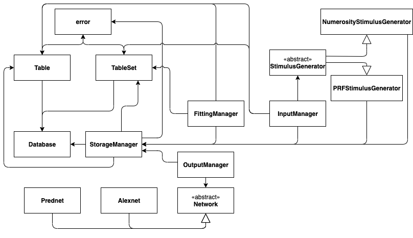
Module diagram
The following figure shows the relations between submodules. Closed arrows represent that a module uses another module somewhere in its functions. Open arrows represent inheritance. To lookup the modules, you can click through them in the sidebar.
View Source
"""
.. include:: ./introduction.md
.. include:: ./getting_started.md
.. include:: ./doc_neural_network.md
.. include:: ./doc_stimulus_set.md
.. include:: ./doc_module_diagram.md
"""
__docformat__ = "google"
__version__ = "1.0.2"

from .storage import *
from .fitting_manager import FittingManager
from .input_manager import *
from .output_manager import *

from .networks import *
from .stimulus_generator import *
from .statistics_helper import *